Introducing slxr: A tool for implementing Spatial-X models

A new R package for Spatial-X (SLX) regression models—variable-specific weights matrices, tidy effects decomposition, and no matrix inversion required.

Spatial econometrics has significant startup costs. If you’ve taken a course or read a textbook chapter on the subject, odds are you learned SAR first, SDM second, and the Spatial-X (SLX) model (if at all) as a footnote on the way to something fancier. That’s backwards. SLX is the simplest of the three, it has a closed-form interpretation, and for a huge share of applied problems in political (and social) science it is exactly the model you want.

slxr is a new R package I built to make SLX the first thing you reach for instead of the last. Install it, write a formula, get a fitted model.¹

install.packages("slxr")

The SLX model in basic terms

An SLX model is just OLS with spatial lags of your covariates on the right-hand side. If W is a spatial weights matrix, you’re fitting y = Xβ + WXθ + ε. That’s it. No lagged y, no simultaneity, no likelihood maximization, no simulation to get effects out. The direct, indirect, and total effects of any covariate are simple functions of β and θ, and they are readable straight off the coefficient table.

The upshot: SLX gives you spatial spillovers without giving up the interpretability of a linear model. For most applied questions where you actually care about where things spill over to rather than whether there’s autocorrelation left in your residuals, that’s a trade worth considering.

The paper that inspired this package

slxr is the software counterpart to Wimpy, Whitten, and Williams (2021), the Journal of Politics piece my coauthors and I wrote to make the case for SLX as the default starting point for spatial work in political science. That paper had three moving parts.

A literature review. We went through every paper in the discipline that used spatial methods through 2015 and coded what the authors’ theories actually claimed versus what their models implicitly imposed. The mismatch was striking: The SAR model, which assumes global dependence, feedback, and infinite-order spillovers—was used in roughly 73% of studies, but fewer than 10% of those studies articulated a theory that was genuinely global. Most theories were about neighbors affecting neighbors. We argue those theories fit SLX, not SAR.

A Monte Carlo. When the true data-generating process was SAR, a simple SLX model augmented with W² and W³ terms recovered the direct, indirect, and total effects at rates comparable to SAR itself. When the true DGP was SLX, however, SAR routinely found “phantom” higher-order and feedback effects that were not in the data, and the bias got worse under spatial heterogeneity (where different covariates flow through different networks). The asymmetry matters. The cost of using SLX when you should have used SAR is small; the cost of using SAR when you should have used SLX is not.

An application. We looked at countries’ defense burdens (operationalized as military spending as a share of GDP) from 1953 to 2008 and asked whether spatial spillovers in defense spending flowed through one network or several. Using variable-specific weights matrices, we let civil war spill over through contiguity, let interstate war spill over through contiguity and alliance ties, and let a country’s own lagged defense burden propagate through contiguity and shared defense pacts. The SAR model produces one ρ, and thus it assumes one spatial story for every covariate. The SLX model showed that civil-war spillovers ran negative (a neighbor’s civil war depressed your defense burden), that alliance-mediated spillovers from interstate war ran positive, and that SAR’s single-ρ summary qualitatively reversed one of those patterns. None of that is legible from a single ρ.

The paper closed with four guidelines for applied researchers and an explicit acknowledgment that software accessibility was, at the time, a barrier to widespread adoption. That’s the gap slxr is built to close.

From the paper to the package

The defense-burden are included with the package. Here’s Table 3, Model 3 of the 2021 paper, written in slxr syntax:

library(slxr)
data(defense_burden)

W_contig   <- slx_weights(style = "custom",
                          matrix = defense_burden$W_contig,
                          row_standardize = FALSE)
W_alliance <- slx_weights(style = "custom",
                          matrix = defense_burden$W_alliance,
                          row_standardize = FALSE)
W_defense  <- slx_weights(style = "custom",
                          matrix = defense_burden$W_defense,
                          row_standardize = FALSE)

fit <- slx(
  ch_milex ~ milex_tm1 + log_pop_tm1 + civilwar_tm1 + total_wars_tm1 +
             alliance_us + ch_milex_us + ch_milex_ussr,
  data    = defense_burden$data,
  spatial = list(
    civilwar_tm1   = W_contig,
    total_wars_tm1 = list(contig = W_contig, alliance = W_alliance),
    milex_tm1      = list(contig = W_contig, defense  = W_defense)
  )
)

slx_effects(fit)
slx_plot_effects(fit, types = c("indirect", "total"))

The spatial = list(...) argument is the piece that makes variable-specific W first-class. Each covariate can spill over through its own network — and, as in the milex_tm1 and total_wars_tm1 rows above, through multiple networks at once.

SLX effects decomposition on the defense-burden data.

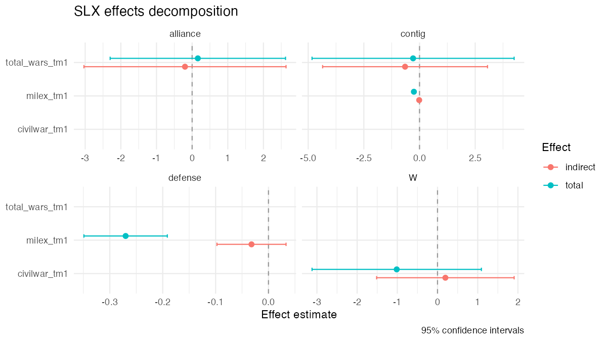
slx_plot_effects() turns that fitted object into the figure above. Each panel is one W; each row is one covariate; each point is the decomposed effect with 95% confidence intervals. The pattern you’re looking at — milex_tm1’s negative spillover through the defense-pact network paired with a civil-war indirect effect that runs opposite the direct — is exactly the kind of heterogeneity a single-ρ SAR model cannot resolve.

What else is inside

Variable-specific W is the headline, but it’s not the whole package. The other features I built slxr around are the ones that are fiddly with existing tools:

• Higher-order lags. W, W², W³, with effects decomposed at each order.
• Temporally-lagged spatial variables (TSLS) for panel data — which is what most applied political science actually looks like.
• Tidy effects. slx_effects() returns a tibble. tidy() and glance() methods plug straight into modelsummary. No more hand-built tables.
• Sensible defaults. Row-standardization, queen contiguity, and a formula interface that doesn’t require you to pre-build a listw object just to find out whether your data file even has coordinates on it.

Why a package instead of replication code

Because replication code works great, but it is often tied to the specific application of the paper. A package turns a method into a tool. slx() works whether you’re studying defense spending, infant mortality, school board decisions, or the diffusion of state policy. The spatial econometrics is the same; only the weights matrix and the covariates change. Wrapping that into one function with a formula interface hopefully allows for easier implementation.

Who this is for

If you’ve ever:

• Fit a SAR model and wished you could just read the spillovers off the coefficients,
• Looked at spdep and bounced off the listw object,
• Wanted to say something substantive about how variable A spills over via one network while variable B spills over via another,
• Or wanted to include a WX term in lm() and been annoyed that there wasn’t a clean way to do it,
• Or even looking to work with spatial econometric theories and data for the first time,

then this package might be for you.

What’s next

Four concrete pieces are on the near-term roadmap:

• A replication vignette for Wimpy, Whitten, and Williams (2021). The full Table 3 end-to-end, from weights matrices to effects plots, in a single Quarto document. The goal is to make the JoP paper something a graduate student can reproduce in an afternoon without ever opening a listw object.
• Diagnostics for W selection. The choice of weights matrix is routinely the most consequential modeling decision in a spatial paper and gets an eyeball test and a sentence. I’d like slxr to include a principled toolkit for comparing competing W specifications. This includes information-criterion ranking, permutation tests, and sensitivity plots. This helps make that choice of W defensible rather than improvised.
• First-class sf pipelines. slx() already accepts sf input, but the round trip from a shapefile to a fitted model still asks more of the user than it should. A sf-aware wrapper that generates contiguity, k-nearest-neighbor, and distance-decay W matrices from a geometry column. This keeps them aligned across panel waves, and I hope it is my next big update
• Panel conveniences. Unbalanced panels work today, but the ergonomics of swapping in year-specific W matrices, handling isolates, and comparing time-invariant vs. time-varying connectivity can be much better than they are.

If any of these would unblock your work, or if you have a use case I haven’t anticipated, the GitHub issue tracker is open and pull requests are welcome. The package is MIT-licensed.

If you just want to try it, the whole thing is one install away:

install.packages("slxr")

Let me know what you think.

Footnotes

1. I built this with scaffolding and testing help from Claude Code. It helped me turn the working development version I had on my Github to something that is now on CRAN.